Bootstrapped White's test for checking homoskedasticity in small samples

I came across this paper where the authors developed a bootstrapped version of the well-known White test. This test checks whether the variance of the residuals in a linear regression model is constant (homoskedasticity). Remember that this is one of the assumptions for a linear regression model to be valid.

The test statistic can be formulated as:

where \(n\) is the number of observations and \(R^2\) is the R-squared of the auxiliary regression of the residuals against fitted values (further details for example here). This test statistic follows a Chi-squared distribution with K-1 degrees of freedom, where K is the number of estimated parameters in the auxiliary regression.

One of the main drawbacks of this method is that it usually performs poorly in small sample sizes, resulting in poor statistical power.

Let’s simulate some fake data that suffer from heteroskedasticity:

# Seed and packages
set.seed(1)
pkgs <- c("dplyr", "tidyr", "ggplot2")
invisible(lapply(pkgs, require, character.only = TRUE))

# Set sample size 
n <- 60
# Generate heteroscedastic data
y <- 1:n
sd <- runif(n, min = 0, max = 4)
error <- rnorm(n, 0, sd*y) 
X <- y+error 
df <- data.frame(y, X)

ggplot(df, aes(y, X)) + 
  geom_point() +
  theme_minimal() +
  labs(title = 'Heteroskedastic data') +
    theme(plot.title = element_text(size=15))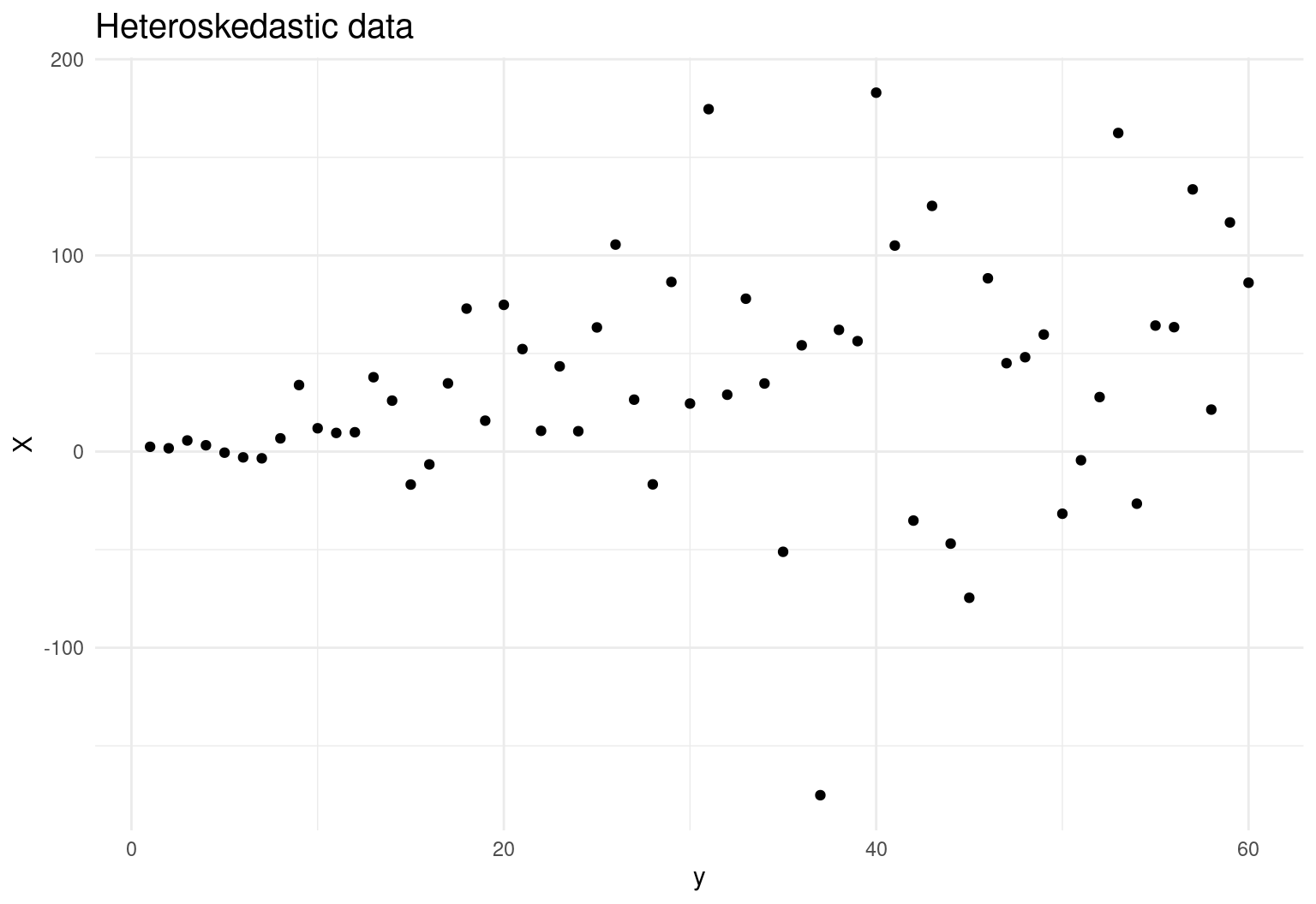 

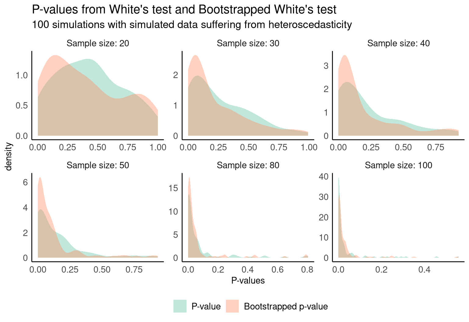
Let’s now run 100 simulations with several sample sizes and compute the p-values for the original test and the bootstrapped version linked above. Sorry in advance for the ugly code:

tst <- tibble()

# For k samples size
for (k in c(20,30,40,50,80,100)) {

  pvalues_orig <- vector('numeric')
  pvalues_boot <- vector('numeric')
  
  for (j in 1:100) {
    
    # Set sample size 
    n <- k
    # Generate heteroscedastic data
    y <- 1:n
    sd <- runif(n, min = 0, max = 4)
    error <- rnorm(n,0,sd*y) 
    X <- y+error
    
    df <- data.frame(y, X)
    
    
    # White test
    m <- lm(y ~ X, data = df)
    u2 <- m$residuals^2
    y <- fitted(m)
    Ru2 <- summary(lm(u2 ~ y + I(y^2)))$r.squared
    LM <- nrow(df)*Ru2
    p.value <- 1-pchisq(LM, 2)
    pvalues_orig <- c(pvalues_orig, p.value)
    
    
    # Bootstrapped White test
    W <- vector(mode = 'numeric')
    bcount <- 0
  
    for (i in 1:1000) {
      # Paper's methodology
      linfit <- lm(y ~ X, data = df)
      pred <- fitted(linfit)
      res <- residuals(linfit)
      var_res <- summary(linfit)$sigma^2
      bootstrapped_error <- var_res * rnorm(n = nrow(df), mean = 0, sd = 1)
      df$new_y <- df$y + bootstrapped_error
      m <- lm(new_y ~ X, data = df)
      Ru2 <- summary(lm(m$residuals^2 ~ fitted(m) + I(fitted(m)^2)))$r.squared
      LM_b <- nrow(df)*Ru2
      
      # compute p-value
      if(abs(LM_b) >= abs(LM)) {
        bcount <- bcount + 1
      }
      
      W[i] <- LM_b
    }
    
    pvalues_boot <- c(pvalues_boot, bcount/1000)
    
  }
  
  # final data.frame
  tst <- bind_rows(tst, 
                   tibble(
                     sample_size = k,
                     pvalues_boot = pvalues_boot,
                     pvalues = pvalues_orig))
  
}

And finally, this is the result, which shows —as the authors state— an improvement in the outcome for small samples.